Load_clean

Part 1. Cleaning the database

R code block:

library(readr)
NY <- read_delim("C:/Users/DDD/Desktop/NY.csv", ";", escape_double = FALSE,
                 trim_ws = TRUE)
NY = ny
library(dplyr)
attach(NY)

cleaning data

Due to the existence of N/A in price (our dependent variable, we fill them with the mean of the variable).

rider$price_1 <- ifelse(is.na(rider$price), mean(rider$price, na.rm=T), rider$price)
rider$longitude <- ifelse(is.na(rider$longitude), mean(rider$longitude, 
                                                       na.rm=T), rider$longitude)
rider$latitude <- ifelse(is.na(rider$latitude), mean(rider$latitude, 
                                                     na.rm=T), rider$latitude)

Making dummy variables for source and destination variables

ri <- fastDummies::dummy_cols(rider, select_columns = c('source',"destination"))
ri <-  select(ri, -c('price'))
ri$id <- 1 

NY %>% count(surge_multiplier, sort=T)
# For the database of Uber, we found that they do not consider the 'surge_multiplier'
# variable to define its price, while for Lyft, indeed they consider the 'surge_multiplier'
# but only for the distance, it is, the 'surge_multiplier' is related to the distance of the trip.

NY %>% select(starts_with('source_')) -> so
NY %>% select(starts_with('destination_')) -> de
dateOnly <- as.Date(rider$datetime, "%d/%m/%Y")
dae <- weekdays(dateOnly) 
da <- as.data.frame(dae)

data.frame(c(so, de)) -> x1
data.frame(c(x, x1, da)) -> ny

write.csv(ny,'ny.csv')

After we cleaned the data, we decided to save the final datafile as csv and reload it again, now the database occupaies less space, and it is the definitive version.

Create Training and Test data -

NY %>% select(-c('id', 'month', 'day','hora')) ->NY

NY %>% filter(cab_type == 'Lyft') -> lyft
NY %>% filter(cab_type == 'Uber') -> uber
uber <-within(uber, rm('cab_type'))
lyft <-within(lyft, rm('cab_type'))

We proceed to remove the outliers of the database for a better estimation

library(data.table)
outlierReplace = function(dataframe, cols, rows, newValue = NA) {
    if (any(rows)) {
        set(dataframe, rows, cols, newValue)
    }
}

NY= outlierReplace(NY, "price", which(NY$price >40), NA)
NY = na.omit(NY)
NY = NY

lyft= outlierReplace(lyft, "price", which(lyft$price >40), NA)
lyft = na.omit(lyft)

uber= outlierReplace(uber, "price", which(uber$price >40), NA)
uber = na.omit(uber)

set.seed(45)  
training_u <- sample(1:nrow(uber), 0.7*nrow(uber))  
trainub <- uber[training_u, ]
testub  <- uber[-training_u, ]

set.seed(45)  
training_ly <- sample(1:nrow(lyft), 0.7*nrow(lyft))  
trainly <- lyft[training_ly, ]
testly <- lyft[-training_ly, ]

lyft %>% count(surge_multiplier, sort=T)

Mean Tables

table(month,cab_type)

mean(lyft$price)
mean(uber$price)

numeric <- NY %>% select_if(is.numeric)
numeric %>% as.matrix() %>% cor() %>% .[,"price"] %>% sort(decreasing = T) -> corr
corr %>% as.table() -> corr
corr

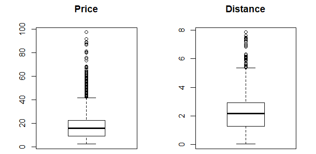
par(mfrow=c(1, 2))  
boxplot(NY$price, main="Price", sub=paste("Outlier rows: ", 
           boxplot.stats(NY$price)$out))  # box plot for 'speed'
boxplot(NY$distance, main="Distance", sub=paste("Outlier rows: ", 
           boxplot.stats(NY$distance)$out))  # box plot for 'distance'

Here’s the Boxplot:

Some graphs

library(dplyr)
library(ggplot2) 

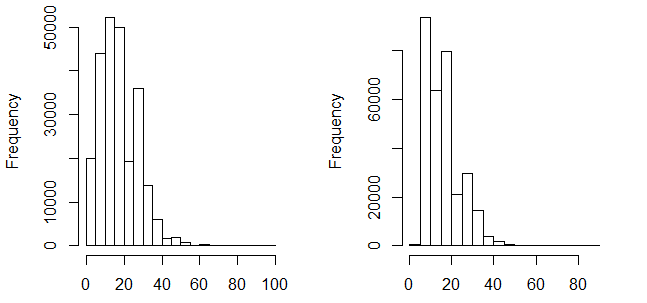
hprice <- ggplot(NY, aes(x=price)) +
  ggtitle("Price histogram") +
  theme_fivethirtyeight() +
  geom_histogram(color="black", fill="coral4")

hdist <- ggplot(NY, aes(x=distance)) +
  ggtitle("Distance histogram") +
  theme_fivethirtyeight() +
  geom_histogram(color="black", fill="coral")

hprice
hdist

boxplot(price ~ cab_type, data = NY, col = "red")

Here’s the price histogram:

Correlation tables

library(corrplot)

nNY <- NY %>% select(price:visibility)
nNY <- nNY %>% select_if(is.numeric)

cor <- round(cor(nNY),2)  
corrplot(cor, method="number", type="upper", tl.cex = 0.6)

Finally some graphs in ggplot

ggplot(NY, aes(x=longitude, y=latitude)) +
+ geom_hex(bins=12, show.legend = T)+ ggtitle('Sources and Destinations')

ggplot(NY, aes(x=longitude, y=latitude)) +
  geom_hex(hbin=12)+ ggtitle('Sources and Destinations')+
  ggtitle('Sources and Destinations')

NY %>% group_by(day) %>% summarize(n=n()) %>%
  ggplot(aes(x=day,y=n)) + geom_point() + 
  geom_line(aes(group=1), linetype='dotted')+
  ylab('Trips')+xlab('Day')+
 ggtitle('Trips by day')
 
 tema = theme(
  axis.title.x = element_text(size = 8),
  axis.text.x = element_text(size = 8),
  axis.title.y = element_text(size = 10))

ggplot(data = rider, mapping = aes(x = source, y = price)) +
  geom_boxplot() + tema + ggtitle('Prices by sources')

This is the end or part 1.