Fluctuations in coin tossing
Fluctuations in coin tossing
The ideal coin-tossing game will be described in the terminology of random walks which is better suited for generalizations. For the geometric description it is convenient to pretend that tossings are performed at a uniformed rate so that the nth trial occurs at epoch p.
We denote individual step generically by X1, X2, …. Xn, and the positions by S1 and S2. Thus
Sn = X1 + X2 + …. Xn, and S0 = 0
For the probability we write
The last binomial coefficient could be expressed as Stirling’s formula
Last visit and long leads
In a long coin-tossing the law of averages ensure that in the game each player will be on the winning side for about half of the time. For this experiment we simulate random coin-tossings and observe that the number of the last trial at which the accumulated number of head and tails were equal, denoted by 2k (0 < k < n).
Symmetry implies that the inequalities k > n/2 and k < n/2 are equally likely.
Suppose we play a game of 10,000 repetitions for each player (we have 2).
import numpy as np

#probability of heads vs. tails. This can be changed.
probability = .5
#num of flips required. This can be changed.
n = 10000

#initiate array
play_1 = np.arange(n)
play_2 = np.arange(n)

def coinFlip(p):
    #perform the binomial distribution (returns 0 or 1)
    result = np.random.binomial(1,p)
    #return flip to be added to numpy array
    return result

for i in range(0, n):
    play_1[i] = coinFlip(probability)
    # i+=1
    play_2[i] = coinFlip(probability)
    i+=1
probability is set to  0.5
Tails = 0, Heads = 1:  [0 1 1 ... 0 0 0]

Player One:
Head Count:  4961
Tail Count:  5039

Player Two
Head Count:  4920
Tail Count:  5080
As we can see from the previous results, in this example, Player 1 has a higher head count, while the opposite for Pkayer 2.
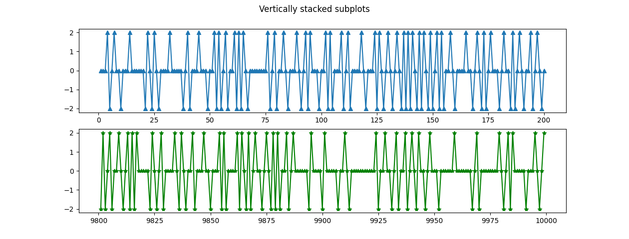
Fig. 1
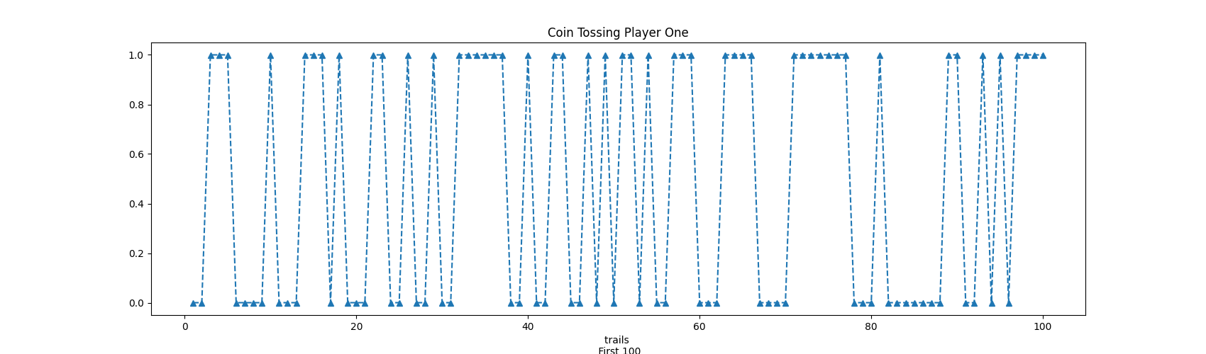
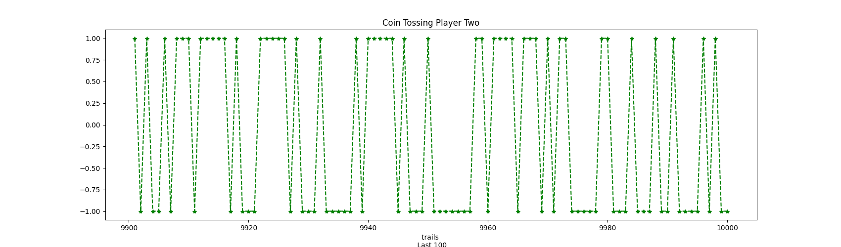
Fig 1.2
Finding k -equality number-
We defined k as the accumulated numbers of heads and tails were equal. We found that all these position are even numbers (python position starts at 0).
[   1,   47,   53,   55, 2725, 2727, 2729, 3381, 3441, 3443, 3463,
        3467, 3469, 3477, 3479, 3483, 3485, 3487, 3489, 3491, 3503, 3505,
        3507, 3509, 3517, 3519, 3521, 3523, 3525, 3527, 3529, 5325, 5329,
        5337, 5341, 5393, 5445, 5451, 5453, 5455, 5457, 5459, 5481, 5485,
        5489, 5491, 5493, 5723, 5725, 5729, 5731, 5733, 5763, 5769, 6199,
        6201, 6205, 6217, 6221, 6227, 6253, 6273, 6275, 6279, 6347, 6361,
        6363]
K for Player Two
[   3,    5,   53,   69,   71,  101,  103,  105,  107,  109,  111,
         113,  121,  225,  229,  231,  251,  253,  257,  277,  555,  557,
         559,  561,  995,  997,  999, 1001, 1003, 1007, 1023, 1033, 1035,
        1037, 1039, 1041, 1043, 1049, 1349, 1351, 1499, 1503, 1507, 1511,
        1513, 1515, 1517]
As we can see the equalization number appears more times for Player one (67 cases), while Player two has a small number of coincidences, only 47. From this result, we can assume that the game was more equal for Player 1, this also can be verified as the number of positions increases, higher than n/2 and lower than the last third. However, we can see that equality were considerably lower for Player 2.
Concluding, we can see that we cannot judge the luck of Player 1 and 2 equally, even at random events one has the chances to succeed more.
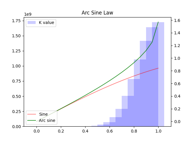
Arc sine law for last visits
The probability that up to and including epoch 2n the last visit to the origin occurs at epoch 2k is given by:
We see that as k increases also increases the probability, also we can see that it is almost similar to an arc sine distribution of k values as the values of k and sample (n) increases.
For this point, we will use a simulation with 20 observations.
import math

n = 20
k = [0,1,2,3,4,5,6,7,8,9,10,11,12,13,14,15,16,17,18,19,20]
k1 = (np.linspace(0,1,21))
distr = [0]*21
out_arc = [0]*21

out_array1 = np.sin(k1)
out_array2 = np.arcsin(k1)


def arc(k):
    #perform the binomial distribution (returns 0 or 1)
    result = (math.comb(2*n,k))/(2**2*n)
    #return flip to be added to numpy array
    return result

for i in (np.int64((k))):
    distr[i] = arc(i)
    out_arc[i] = np.sin(i)
    i+=1


import matplotlib.pyplot as plt
import matplotlib.patches as mpatches

fig, ax1 = plt.subplots()
ax2 = ax1.twinx()
ax2.plot(k1, out_array1, color = 'red', alpha = 0.5, label='Sine')
ax1.bar(k1, distr,color = 'b', alpha = 0.2, width=.1, label='K value')
ax2.plot(k1, out_array2,color = 'g', alpha = 0.8, label='Arc sine')
b_patch = mpatches(color='blue', alpha = 0.8, label='K value')
plt.legend(loc='lower left')
ax1.legend(handles=[b_patch])
plt.title('Arc Sine Law')
plt.show()
Fig 2
from astropy.table import QTable, Table, Column
from astropy import units as u

t = QTable()
t['k'] = k
t['a'] = distr
t
Table 1. The discrete arc sine distribution of order n.
| K | \alpha_{2k,20} |
|---|---|
| 1 | 3.637978807091713e-11 |
| 5 | 5.98454789724201e-07 |
| 10 | 0.0007709427591180429 |
| 15 | 0.03658473820541985 |
| 19 | 0.11940065487578977 |
As we can see as n increases also the value of k, possibly reflecting the notion that as n increases in a coin-tossing game, one of the players will remain more time on one side, and the other on the other side. This is half-truth, due to two reason, we can see from the above example that Player 1 has more head counts than Player 2, but contrary to the theory, from Figure 3, we saw that the “arc sine distribution” appears when n starts increasing.
Changes of signs
Lastly, considering the above example of coins tossing. The number of changes in a n trials game, we should expect a number of changes (opposite sides) around the square root of n.
However, as long the number of epochs (r) increases the probability of the number changes should decrease.
As we see the probability has a Normal approximation:
prl = []
lr = [5,10,20,30]

def pr(i):
    res = (1/np.sqrt(math.pi*i))
    return res

for i in lr:
    prl.append(pr(i))
    i +=1

# Table of probabilities
t = QTable()
t['k'] = [5,10,20,30]
t['a'] = np.round(pr,3)
Table 2. Table of probabilities of no change
| r | pr |
|---|---|
| 5 | 0.252 |
| 10 | 0.178 |
| 20 | 0.126 |
| 30 | 0.103 |
Counting the number of changes in the tossing coins example
total = [0]*9999
for ele in range(1, len(play_1)):
    total[ele]= play_1[ele+1] - play_1[ele]
    ele+=1

total_2 = [0]*9999
for ele in range(1, len(play_2)):
    total_2[ele]= play_1[ele+1] - play_1[ele]
    ele+=1

print('Positive side changes',total.count(1))
print('Negative side changes',total.count(-1))
PLAYER ONE:
Positive side changes 2497
Negative side changes 2498

PLAYER TWO:
Positive side changes 2477
Negative side changes 2476
For player 1
import collections

ps1 = collections.Counter(play_1)[0]
pn1 = collections.Counter(play_1)[1]
print('Number of times in the positive side',ps1,';',ps1/n, 'percentage of time')
print('Number of times in the negative side',pn1,';',pn1/n, 'percentage of time')
Number of times in the positive side 4962 ; 0.4962 percentage of total time
Number of times in the negative side 5038 ; 0.5038 percentage of total time
Player 2
ps2 = collections.Counter(play_2)[0]
pn2 = collections.Counter(play_2)[1]
print('Number of times in the positive side',ps2,';',ps2/n, 'percentage of time')
print('Number of times in the negative side',pn2,';',pn2/n, 'percentage of time')
Number of times in the positive side 4995 ; 0.4995 percentage of total time
Number of times in the negative side 5005 ; 0.5005 percentage of total time
Fig 3