Gbm

Gradient Boosting Machine (GBM)

Whereas random forests build an ensemble of deep independent trees, GBMs build an ensemble of shallow and weak successive trees with each tree learning and improving on the previous. When combined, these many weak successive trees produce a powerful “committee” that are often hard to beat with other algorithms. For this section, we also use the same split of Random Forest exercise that is 260,000 observations. For this procedure we use the ‘gbm library’.

library(gbm)
library(dplyr)
library(Metrics)
library(ggthemes)
library(scales)
library(ggplot2)

Since gbm is so flexible, we choose as maximum number of trees 700, since we believe it was sufficient to achieve a low error and we also adjust the estimation with different selections of shrinkage (0.01, 0.02, and 0,03). In Table 5A, we see that the best tree selection which produces the smallest error is with shrinkage equal to 0.03, where for both cases, it has the smallest CV error.

UBER

set.seed(45)
gb01 = gbm(price ~., data=trainub, interaction.depth=4,shrinkage= 0.03,n.trees =700,
           distribution='gaussian', cv.folds = 5 )
print(gb01)
sqrt(min(gb01$cv.error))
set.seed(45)
gb02 = gbm(price ~., data=trainub, interaction.depth=4,shrinkage= 0.05,n.trees =700,
           distribution='gaussian', cv.folds = 5 )
print(gb02)
sqrt(min(gb02$cv.error))
set.seed(45)
gb03 = gbm(price ~., data=trainub, interaction.depth=4,shrinkage= 0.01,n.trees =700,
           distribution='gaussian', cv.folds = 5 )
print(gb03)
sqrt(min(gb03$cv.error))

par(mfrow=c(1,2))
par(mar = c(5, 8, 1, 1))
summary(gb03, cBars = 10, method = relative.influence,las = 1,
        cex.names=.8, cex.axis=1)
gbm.perf(gb03, method = "cv")

par(mfrow=c(1,2))
par(mar = c(5, 8, 1, 1))
gbm.perf(gb01, method = "cv")
gbm.perf(gb02, method = "cv")

LYFT

set.seed(45)
gb2=gbm(price ~., data=trainly, interaction.depth=4,shrinkage=0.01,n.trees =700,
        distribution='gaussian', cv.folds = 5)
print(gb2)
sqrt(min(gb2$cv.error))
set.seed(45)
gb21=gbm(price ~., data=trainly, interaction.depth=4,shrinkage=0.03,n.trees =700,
         distribution='gaussian', cv.folds = 5)
print(gb21)
sqrt(min(gb21$cv.error))
set.seed(45)
gb22=gbm(price ~., data=trainly, interaction.depth=4,shrinkage=0.05,n.trees =700,
         distribution='gaussian', cv.folds = 5)
print(gb22)
sqrt(min(gb22$cv.error))

par(mfrow=c(1,2))
par(mar = c(5, 8, 1, 1))
summary(gb2, cBars = 10, method = relative.influence,las = 1,
        cex.names=.7, cex.axis=1,)
gbm.perf(gb2, method = "cv")

par(mfrow=c(1,2))
par(mar = c(5, 8, 1, 1))
gbm.perf(gb21, method = "cv")
gbm.perf(gb22, method = "cv")

Here’s the Table for shrinkage, best tree and CV error - Full model selection:

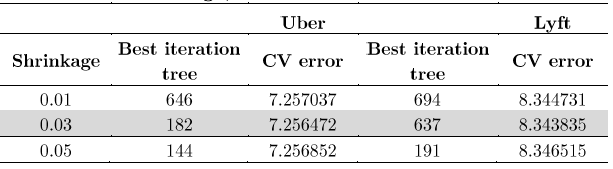
Below we show some of the figures of the estimation. Although Uber estimation requires less number of trees get a minor CV error, Lyft figures shows that it require 637 trees to achieve a lower error, however both were under a shrinkage of 0.03.

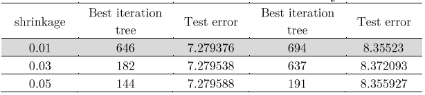
After we realize the estimation of the different models, we proceed to make a Table of with the prediction errors. In that way, as we can assume the models with small prediction error were with a shrinkage equal to 0.01.

Prediction of errors: Full model

Finally, predict.gbm() function allows to generate the predictions out of the data. One important feature of the gbm’s predict is that the user has to specify the number of trees. Since there is no default value for “n.trees” in the predict function, it is compulsory for the modeller to specify one. Since we have figured out the optimum number of trees by performing early stopping, we will use the optimum values for specifying the “n.trees” argument. I have used the optimum solution based on the cross validation technique as cross validation usually outperforms the OOB method on large datasets. One another argument that the user can specify in the predict function is the type, which controls the type of output generated from the function. In other words, type refers to the scale on which gbm makes predictions.

UBER

predgb01 = predict(gb01, testub, n.trees = 182, type = 'response')
rmse_gb01 <- Metrics::rmse(actual = testub$price, predicted = predgb01)
print(rmse_gb01)
predgb02 = predict(gb02, testub, n.trees = 144, type = 'response')
rmse_gb02 <- Metrics::rmse(actual = testub$price, predicted = predgb02)
print(rmse_gb02)
predgb03 = predict(gb03, testub, n.trees = 646, type = 'response')
rmse_gb03 <- Metrics::rmse(actual = testub$price, predicted = predgb03)
print(rmse_gb03)

LYFT

predgb2 = predict(gb2, testly, n.trees = 694, type = 'response')
rmse_gb2 <- Metrics::rmse(actual = testly$price, predicted = predgb2)
print(rmse_gb2)
predgb21 = predict(gb21, testly, n.trees = 230, type = 'response')
rmse_gb21 <- Metrics::rmse(actual = testly$price, predicted = predgb21)
print(rmse_gb21)
predgb22 = predict(gb22, testly, n.trees = 143, type = 'response')
rmse_gb22 <- Metrics::rmse(actual = testly$price, predicted = predgb22)
print(rmse_gb22)

Here’s the Table for Prediction errors - Full model:

Once we have our selection, that is we selected the model with less prediction error, we show the relative influence table and chart for both firms.

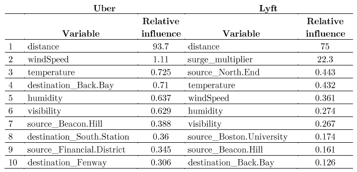
Here’s the Top 10 drives of pricing - Uber and Lyft (Full model):

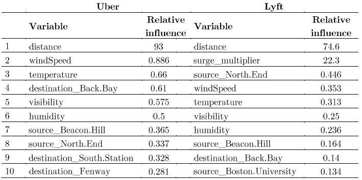
Analyzing the gbm results and compared with those from Random Forest, this time we see that the output includes weather features, for example windspeed, temperature, visibility and humidity are among the 10 top drivers of pricing, and Boston University remains as a powerful predictor.

Second iteration: selecting the first 14 more important variables

set.seed(45)
gb1=gbm(price ~distance + windSpeed+temperature+visibility+humidity+precipIntensity+
    destination_Back.Bay+source_Beacon.Hill+ source_North.End + destination_Fenway+
    source_Back.Bay+source_Northeastern.University+destination_South.Station+
    source_Financial.District,  data=trainub, interaction.depth=4,shrinkage= 0.01,
    n.trees =700, distribution='gaussian', cv.folds = 5)
print(gb1)
sqrt(min(gb1$cv.error))

par(mfrow=c(1,2))
par(mar = c(5, 8, 1, 1))
summary(gb1, cBars = 10, method = relative.influence,las = 1,
    cex.names=.7, cex.axis=1)
gbm.perf(gb1, method = "cv")

set.seed(45)
gb12=gbm(price ~distance + windSpeed+temperature+visibility+humidity+precipIntensity+
     destination_Back.Bay+source_Beacon.Hill+ source_North.End + destination_Fenway+
     source_Back.Bay+source_Northeastern.University+destination_South.Station+
     source_Financial.District, data=trainub, interaction.depth=4,shrinkage= 0.03,n.trees =700,
     distribution='gaussian', cv.folds = 5)
print(gb12)
sqrt(min(gb12$cv.error))

set.seed(45)
gb13=gbm(price ~distance + windSpeed+temperature+visibility+humidity+precipIntensity+
  destination_Back.Bay+source_Beacon.Hill+ source_North.End + destination_Fenway+
  source_Back.Bay+source_Northeastern.University+destination_South.Station+
 source_Financial.District,  data=trainub, interaction.depth=4,shrinkage= 0.05,
 n.trees =700, distribution='gaussian', cv.folds = 5)
print(gb13)
sqrt(min(gb13$cv.error))

par(mfrow=c(1,2))
par(mar = c(5, 8, 1, 1))
gbm.perf(gb12, method = "cv")
gbm.perf(gb13, method = "cv")

Second iteration LYFT: 14 more important variables.

set.seed(45)
gb21L=gbm(price ~ surge_multiplier+distance +windSpeed+visibility+temperature+
    humidity+source_North.End+precipIntensity +destination_Back.Bay+
    source_Boston.University+source_Beacon.Hill+source_North.Station+
    source_Financial.District+source_Back.Bay, data=trainly,
    interaction.depth=4,shrinkage=0.01,n.trees =700,
     distribution='gaussian', cv.folds = 5)
print(gb21L)
sqrt(min(gb21L$cv.error))

set.seed(45)
gb22L=gbm(price ~ surge_multiplier+distance +windSpeed+visibility+temperature+
   humidity+source_North.End+precipIntensity +destination_Back.Bay+
  source_Boston.University+source_Beacon.Hill+source_North.Station+
   source_Financial.District+source_Back.Bay,data=trainly, 
  interaction.depth=4,shrinkage=0.03,n.trees =700,
   distribution='gaussian', cv.folds = 5)
print(gb22L)
sqrt(min(gb22L$cv.error))

set.seed(45)
gb23L=gbm(price ~ surge_multiplier+distance +windSpeed+visibility+temperature+
 humidity+source_North.End+precipIntensity +destination_Back.Bay+
source_Boston.University+source_Beacon.Hill+source_North.Station+
source_Financial.District+source_Back.Bay, data=trainly, interaction.depth=4,
shrinkage=0.05,n.trees =700, distribution='gaussian', cv.folds = 5)
print(gb23L)
sqrt(min(gb23L$cv.error))

par(mfrow=c(1,2))
par(mar = c(5, 8, 1, 1))
summary(gb21L, cBars = 10, method = relative.influence, 
        las = 1,cex.names=.7, cex.axis=1)
gbm.perf(gb21L, method = "cv")

par(mfrow=c(1,2))
par(mar = c(5, 8, 1, 1))
gbm.perf(gb22L, method = "cv")
gbm.perf(gb23L, method = "cv")

Since with shrinkage 0.01, the prediction error is smaller compared with other we decided to consider this model (and its variables) for the next step of this exercise, that is we consider the 14 variables with more relative influence in the model, in this last step we do not consider the latitude and longitude variables since we believe they are already represented in their destinations and sources.

Here’s the Table for Shrinkage, best tree and CV error: 14 variables

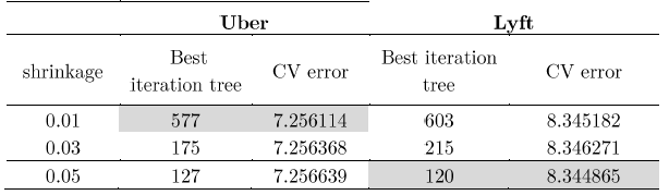
This time, the results are different for Lyft, the minor CV error is under 120 trees and with a shrinkage equal to 0.05. Uber achieves the smallest CV error with shrinkage of 0.01.

predictions: Second iteration

predgb1 = predict(gb1, testub, n.trees = 577, type = 'response')
rmse_gb1 <- Metrics::rmse(actual = testub$price, predicted = predgb1)
print(rmse_gb1)
predgb12 = predict(gb12, testub, n.trees = 175, type = 'response')
rmse_gb12 <- Metrics::rmse(actual = testub$price, predicted = predgb12)
print(rmse_gb12)
predgb13 = predict(gb13, testub, n.trees = 127, type = 'response')
rmse_gb13 <- Metrics::rmse(actual = testub$price, predicted = predgb13)
print(rmse_gb13)

predgb21 = predict(gb21L, testly, n.trees = 603, type = 'response')
rmse_gb21 <- Metrics::rmse(actual = testly$price, predicted = predgb21)
print(rmse_gb21)
predgb22 = predict(gb22L, testly, n.trees = 215, type = 'response')
rmse_gb22 <- Metrics::rmse(actual = testly$price, predicted = predgb22)
print(rmse_gb22)
predgb23 = predict(gb23L, testly, n.trees = 120, type = 'response')
rmse_gb23 <- Metrics::rmse(actual = testly$price, predicted = predgb23)
print(rmse_gb23)

UBER: Variable importance

ubereff <- tibble::as_tibble(gbm::summary.gbm(gb1, plotit = F))
ubereff %>% utils::head(10)

ubereff %>% 
    # arrange descending to get the top influencers
    dplyr::arrange(desc(rel.inf)) %>%
    # sort to top 10
    dplyr::top_n(10) %>%
    # plot these data using columns
    ggplot(aes(x = forcats::fct_reorder(.f = var, .x = rel.inf), y = rel.inf, fill = rel.inf)) +
    geom_col() +
    # flip
    coord_flip() +
    # format
    scale_color_brewer(palette = "Dark2") +
    theme_fivethirtyeight() +
    theme(axis.title = element_text()) + 
    xlab('Features') +
    ylab('Relative Influence') +
    ggtitle("Top 10 Drivers of Uber pricing")

Predicted prices for Uber

testub$predicted <- base::as.integer(predict(gb1, newdata = testub, n.trees = 577))
ggplot(testub) + geom_point(aes(y = predicted, x = price, color = predicted - price), alpha = 0.7) +
    theme_fivethirtyeight() +
    # strip text
    theme(axis.title = element_text()) + 
    # add format to labels
    scale_x_continuous(labels = comma) +
    scale_y_continuous(labels = comma) +
    # add axes/legend titles
    scale_color_continuous(name = "Predicted - Actual", labels =comma) +
    ylab('Predicted prices') +
    xlab('Actual prices') +
    ggtitle('Predicted vs Actual Uber prices') 

Here’s the Top 10 drives of pricing - Uber and Lyft: selected variables

LYFT: Variable importance

lyfteff <- tibble::as_tibble(gbm::summary.gbm(gb21L, plotit = F))
lyfteff %>% utils::head(10)

lyfteff %>% 
    # arrange descending to get the top influencers
    dplyr::arrange(desc(rel.inf)) %>%
    # sort to top 10
    dplyr::top_n(10) %>%
    # plot these data using columns
    ggplot(aes(x = forcats::fct_reorder(.f = var, .x = rel.inf), y = rel.inf, fill = rel.inf)) + geom_col() +
    # flip
    coord_flip() +
    # format
    scale_color_brewer(palette = 'Reds') +
    theme_fivethirtyeight() +
    theme(axis.title = element_text()) + 
    xlab('Features') +
    ylab('Relative Influence') +
    ggtitle("Top 10 Drivers of Lyft pricing")

Predicted prices for Lyft

testly$predicted <- base::as.integer(predict(gb1, newdata = testly, n.trees = 603))
ggplot(testly) + geom_point(aes(y = predicted, 
    x = price, color = predicted - price), alpha = 0.7) +
    theme_fivethirtyeight() +
    # strip text
    theme(axis.title = element_text()) + 
    # add format to labels
    scale_x_continuous(labels = comma) +
    scale_y_continuous(labels = comma) +
    # add axes/legend titles
    scale_color_continuous(name = "Predicted - Actual", labels =comma) +
    ylab('Predicted Prices') +
    xlab('Actual Prices') +
    ggtitle('Predicted vs Actual Lyft Prices') 

We present only the top 10 predictors for the sub-sample of 14 variables, as we could imagine the order has changed, still, weather features are present, and some destinations and sources places have changed, for example, we can see that for Uber: source_North.End is not present anymore, and source_Financial.District is among the top 10.

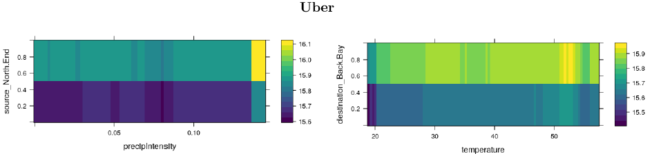
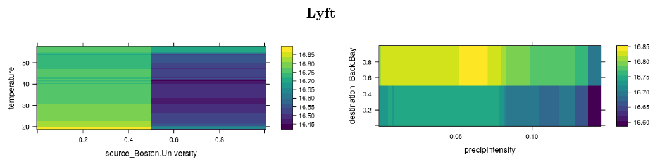
Price response: Two variable interaction

Similarly, we can look at the interaction of two features on prices. Below we can see that prices are more likely to increase in some selected locations, regarding, weather phenomenon, it appears that these have an effect on prices, only when temperatures are lower –less tan 20Fº-, and when the precipitation is really high. But it is clear that the price will change regarding the location.

Responses graphs: Uber

gbm::plot.gbm(gb1, i.var = c(6, 9))
gbm::plot.gbm(gb1, i.var = c(3, 7))
gbm::plot.gbm(gb1, i.var = c(6, 3))

Here’s the interaction effects on pricing - Uber

Responses graphs: Lyft

gbm::plot.gbm(gb21L, i.var = c(10, 5))
gbm::plot.gbm(gb21L, i.var = c(8, 9))
gbm::plot.gbm(gb21L, i.var = c(5, 13))

Here’s the interaction effects on pricing - Lyft

This is the end of part 5.