PCR & PLS
Performing Principal Components Regression (PCR) and Partial Least Squares Regression (PLS) in Python
%matplotlib inline
import pandas as pd
import numpy as np
import matplotlib.pyplot as plt

from sklearn.preprocessing import scale
from sklearn import model_selection
from sklearn.decomposition import PCA
from sklearn.linear_model import LinearRegression
from sklearn.cross_decomposition import PLSRegression, PLSSVD
from sklearn.metrics import mean_squared_error


df = pd.read_csv("D://Gitrepo//Blog//rus2.csv", sep=",")
def clean_dataset(df):
    assert isinstance(df, pd.DataFrame), "df needs to be a pd.DataFrame"
    df.dropna(inplace=True)
    indices_to_keep = ~df.isin([np.nan, np.inf, -np.inf]).any(1)
    return df[indices_to_keep]
dt = df.select_dtypes(include=np.number)
clean_dataset(dt)
dt.head(6)
| total_time | wait_time | surge_multiplier | driver_gender | price_usd | distance_kms | temperature_value | humidity | wind_speed | |
|---|---|---|---|---|---|---|---|---|---|
| 0 | 29 | 7 | 1.0 | 1 | 5.17 | 9.29 | 12 | 0.69 | 4.81 |
| 1 | 26 | 6 | 1.0 | 1 | 4.97 | 9.93 | 10 | 0.70 | 6.53 |
| 2 | 83 | 16 | 1.0 | 1 | 13.01 | 18.01 | 14 | 0.61 | 5.25 |
| 3 | 20 | 6 | 2.9 | 1 | 25.99 | 5.10 | 3 | 0.84 | 0.87 |
| 4 | 49 | 10 | 1.4 | 1 | 13.43 | 21.92 | 3 | 0.90 | 1.61 |
| 5 | 34 | 17 | 1.0 | 1 | 4.06 | 4.88 | 7 | 0.83 | 2.73 |
df[df["ride_hailing_app"] == "Uber"].shape
df[df["ride_hailing_app"] == "Gett"].shape

print(
    "Uber size: ",
    df[df["ride_hailing_app"] == "Uber"].shape,
    "\n Gett size: ",
    df[df["ride_hailing_app"] == "Gett"].shape,
)
Uber size:  (642, 19)
 Gett size:  (36, 19)
y = dt["price_usd"].values
x = dt.drop(["price_usd"], axis=1)
pca = PCA()
X_reduced = pca.fit_transform(scale(x))
pd.DataFrame(pca.components_.T).loc[:5, :5]
# 10-fold CV, with shuffle
n = len(X_reduced)
kf_10 = model_selection.KFold(n_splits=10, shuffle=True, random_state=1)
regr = LinearRegression()
mse = []

# Calculate MSE with only the intercept (no principal components in regression)
score = (
    -1
    * model_selection.cross_val_score(
        regr, np.ones((n, 1)), y.ravel(), cv=kf_10, scoring="neg_mean_squared_error"
    ).mean()
)
mse.append(score)

# Calculate MSE using CV for the 19 principle components, adding one component at the time.
for i in np.arange(1, 20):
    score = (
        -1
        * model_selection.cross_val_score(
            regr,
            X_reduced[:, :i],
            y.ravel(),
            cv=kf_10,
            scoring="neg_mean_squared_error",
        ).mean()
    )
    mse.append(score)

# Plot results
fig = plt.figure()
ax = fig.add_subplot(111)
plt.plot(mse, "-v")
plt.xlabel("Number of principal components in regression")
plt.ylabel("MSE")
plt.title("Price")

ymin = min(mse)
xpos = mse.index(ymin)
xmin = np.arange(1, 20)[xpos]  # min 8

ax.annotate(
    "Min. MSE",
    xy=(xmin, ymin),
    xytext=(xmin, ymin + 2),
    arrowprops=dict(facecolor="red", shrink=0.02),
)

plt.xlim(xmin=-1)
(-1.0, 19.95)
Here’s the plot for the best regression model : 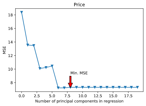
np.cumsum(np.round(pca.explained_variance_ratio_, decimals=3) * 100)

# When M= 5 we get an 80.3%
[23.3, 42.4, 55.4, 67.9, 80.3, 91.6, 98. , 99.9]
## Now let's perform PCA on the training data and evaluate its test set performance:

pca2 = PCA()
# Split into training and test sets
x_train, x_test, y_train, y_test = model_selection.train_test_split(
    x, y, test_size=0.3, random_state=1
)
# Scale the data
x_reduc_train = pca2.fit_transform(scale(x_train))
n = len(x_reduc_train)

# 10-fold CV, with shuffle
kf_10 = model_selection.KFold(n_splits=10, shuffle=True, random_state=1)
mse2 = []

# Calculate MSE with only the intercept (no principal components in regression)
score2 = (
    -1
    * model_selection.cross_val_score(
        regr,
        np.ones((n, 1)),
        y_train.ravel(),
        cv=kf_10,
        scoring="neg_mean_squared_error",
    ).mean()
)
mse.append(score2)

# Calculate MSE using CV for the 19 principle components, adding one component at the time.
for i in np.arange(1, 20):
    score2 = (
        -1
        * model_selection.cross_val_score(
            regr,
            x_reduc_train[:, :i],
            y_train.ravel(),
            cv=kf_10,
            scoring="neg_mean_squared_error",
        ).mean()
    )
    mse2.append(score2)
# Plot results
fig = plt.figure()
ax = fig.add_subplot(111)
plt.plot(mse2, "-v")
plt.xlabel("Number of principal components in regression")
plt.ylabel("Reduced MSE")
plt.title("Price")

ymin = min(mse2)
xpos = mse2.index(ymin)
xmin = np.arange(1, 20)[xpos]  # min 6

ax.annotate(
    "Min. MSE",
    xy=(xmin, ymin),
    xytext=(xmin, ymin + 1),
    arrowprops=dict(facecolor="red", shrink=0.02),
)

plt.xlim(xmin=-1)
(-1.0, 18.9)
Here’s the plot for the best regression model : 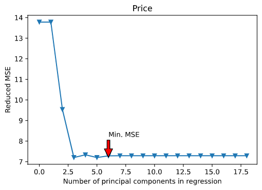
np.cumsum(np.round(pca2.explained_variance_ratio_, decimals=3) * 100)
[ 23.4, 42.5, 55.8, 68.3, 80.7, 92. , 98.3, 100. ]
## We find that the lowest cross-validation error occurs when  M=6  components are used.

x_redu_test = pca2.transform(scale(x_test))[:, :5]

# Train regression model on training data
regr = LinearRegression()
regr.fit(x_reduc_train[:, :5], y_train)

# Prediction with test data
pred = regr.predict(x_redu_test)
mean_squared_error(y_test, pred)
8.909402005123031
from sklearn.pipeline import make_pipeline
from sklearn.preprocessing import StandardScaler

pcr = make_pipeline(StandardScaler(), PCA(n_components=6), LinearRegression())
pcr.fit(x_train, y_train)
pca = pcr.named_steps['pca']
# 6.7.2 Partial Least Squares

n = len(x_train)

# 10-fold CV, with shuffle
kf_10 = model_selection.KFold(n_splits=10, shuffle=True, random_state=1)
pls_mse = []

for i in np.arange(1, 9):
    pls = PLSRegression(n_components=i)
    score = model_selection.cross_val_score(
        pls, scale(x_train), y_train, cv=kf_10, scoring="neg_mean_squared_error"
    ).mean()
    pls_mse.append(-score)
fig = plt.figure()
ax = fig.add_subplot(111)
plt.plot(np.arange(1, 9), np.array(pls_mse), "-v", color="green")
plt.xlabel("Number of principal components in regression")
plt.ylabel("MSE")
plt.title("Price")

ymin = min(pls_mse)
xpos = pls_mse.index(ymin)
xmin = np.arange(1, 9)[xpos]  # min 6

ax.annotate(
    "Min. MSE",
    xy=(xmin, ymin),
    xytext=(xmin, ymin + 0.08),
    arrowprops=dict(facecolor="yellow", shrink=0.02),
)

plt.show()
Here’s the plot for the best regression model : 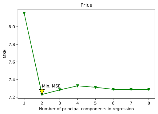
pls = PLSRegression(n_components=2)
pls.fit(scale(x_train), y_train)

mean_squared_error(y_test, pls.predict(scale(x_test)))
9.19707333152056
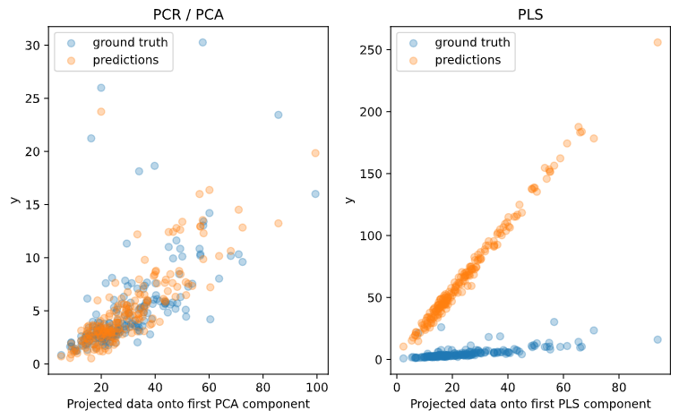
fig, axes = plt.subplots(1, 2, figsize=(8, 5))
axes[0].scatter(pca.transform(x_test)[:,0], y_test, alpha=.3, label='ground truth')
axes[0].scatter(pca.transform(x_test)[:,0], pcr.predict(x_test), alpha=.3,
                label='predictions')
axes[0].set(xlabel='Projected data onto first PCA component',
            ylabel='y', title='PCR / PCA')
axes[0].legend(loc='upper left')

axes[1].scatter(pls.transform(x_test)[:,0], y_test, alpha=.3, label='ground truth')
axes[1].scatter(pls.transform(x_test)[:,0], pls.predict(x_test), alpha=.3,
                label='predictions')
axes[1].set(xlabel='Projected data onto first PLS component',
            ylabel='y', title='PLS')
axes[1].legend()
plt.tight_layout()
plt.show()
Here’s the plot for the best regression model :