Toptal challenge
Pandas and classification exercise
import numpy as np
import pandas as pd
from sklearn.tree import DecisionTreeClassifier
from sklearn.model_selection import train_test_split
from sklearn.metrics import confusion_matrix
from random import randint
from matplotlib import pyplot as plt
import seaborn as sns
For this exercise, it is required to use only three libraries: Pandas, Numpy, and Sklearn -this last one is used for the Decision tree and the confusion matrix-. Additionally, we imported the random and Matplotlib and Seaborn libraries to make the exercise completer and more visual.
To continue we upload both Training and Test databases. For this exercise, it is only required to use the Training Database.
data_test = pd.read_csv('test.csv')
data_train = pd.read_csv('train.csv')
data_train.head(6)
| duration | credit_amount | installment_rate | present_residence | age | existing_credits | dependents | checking_account_status_A12 | checking_account_status_A13 | checking_account_status_A14 | ... | other_installment_plans_A142 | other_installment_plans_A143 | housing_A152 | housing_A153 | job_A172 | job_A173 | job_A174 | telephone_A192 | foreign_worker_A202 | target | |
|---|---|---|---|---|---|---|---|---|---|---|---|---|---|---|---|---|---|---|---|---|---|
| 0 | 36 | 8086.0 | 2.0 | 4.0 | 42.0 | 4.0 | 1 | 1 | 0 | 0 | ... | 0 | 1 | 1 | 0 | 0 | 0 | 1 | 1 | 0 | 1 |
| 1 | 15 | 3812.0 | 1.0 | 4.0 | 23.0 | 1.0 | 1 | 0 | 0 | 1 | ... | 0 | 1 | 1 | 0 | 0 | 1 | 0 | 1 | 0 | 0 |
| 2 | 36 | 2145.0 | 2.0 | 1.0 | 24.0 | 2.0 | 1 | 0 | 0 | 0 | ... | 0 | 1 | 1 | 0 | 0 | 1 | 0 | 1 | 0 | 1 |
| 3 | 12 | 2578.0 | 3.0 | 4.0 | 55.0 | 1.0 | 1 | 0 | 0 | 0 | ... | 0 | 1 | 0 | 1 | 0 | 0 | 1 | 0 | 0 | 0 |
| 4 | 21 | 5003.0 | 1.0 | 4.0 | 29.0 | 2.0 | 1 | 0 | 0 | 1 | ... | 0 | 0 | 1 | 0 | 0 | 1 | 0 | 1 | 0 | 1 |
| 5 | 15 | 2327.0 | 2.0 | 3.0 | 25.0 | 1.0 | 1 | 0 | 1 | 0 | ... | 0 | 1 | 1 | 0 | 1 | 0 | 0 | 0 | 0 | 1 |
6 rows × 49 columns
Modeling on the Training dataset
We constructed a function to split the Database into a Training and Test database, the former one with a size of 30%, and a random state equal to 42 for the reproduction of the results.
def uplo(db):
    y = db['target']
    X = db.drop('target', axis=1)
    xt, xte, yt, yte = train_test_split(X, y, test_size=0.3, random_state=42)
    print('The shape of dataset:', X.shape[0])
    print('The shape of the X dataset:', xt.shape[0])

    return xt,xte,yt,yte
X_train, X_test, y_train, y_test = uplo(data_train)
The shape of dataset: 900
The shape of the X dataset: 630
The dataset has a size of 900 rows and the X_train dataset of size 630.
Correlation matrix
To continue we construct a Correlation Matrix as a way to take the most significant variables with the target variable, this is not required in the exercise.
And as an example, here we consider the 10 most important ones.
corrMatrix = data_train.corr()
print(corrMatrix['target'][:10].sort_values(ascending=False))
duration                       0.223492
credit_amount                  0.168680
checking_account_status_A12    0.116657
installment_rate               0.065554
present_residence              0.007676
dependents                    -0.002630
existing_credits              -0.055938
checking_account_status_A13   -0.082670
age                           -0.097674
checking_account_status_A14   -0.315427
Name: target, dtype: float64
From our the correlation matrix -only considering the the most important 10 variables correlated with target-, we take as important variables: duration and age being the former with the highest positive correlation and the latest with the negative correlation.
col = [ 'target','duration' ,
'credit_amount' ,'checking_account_status_A12' ,
'installment_rate','present_residence',
'dependents','existing_credits','checking_account_status_A13' ,
'age', 'checking_account_status_A14']
corr = data_train[col].corr()

ax = sns.heatmap(  corr,
    vmin=-1, vmax=1, center=0,
    cmap=sns.diverging_palette(20, 200, n=200),
    square=True)

ax.set_xticklabels(ax.get_xticklabels(),
    rotation=45, horizontalalignment='right');
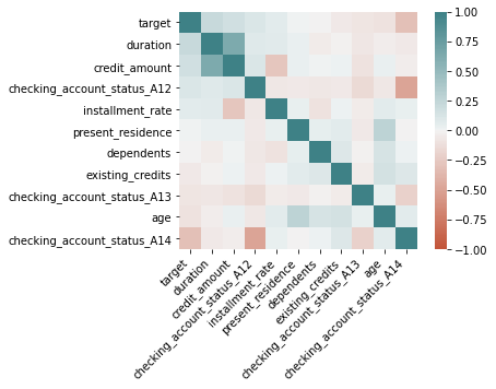
After the correlation matrix, we decided to take two variables that have a considerable impact on the target variable (positive and negative correlation), which are: duration and age.
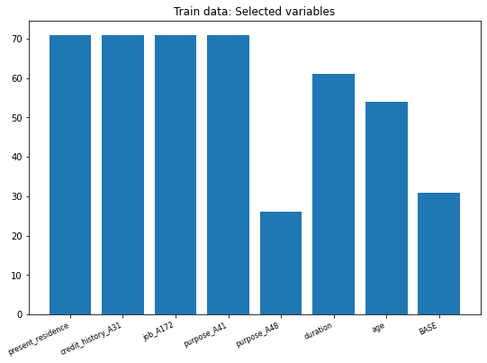
In the next step, we construct an empty list that saves the metrics of the Classifier tree, then we take five random variables from the Train database and add the other selected two correlated variables.
fp = []
nu = [randint(2, 49) for p in range(2, 7)]
nam = list(X_train.columns[nu])
nam.extend(['duration','age'])
nam
From the above results, we can see that were chosen five variables randomly, and duration and age were added too.
['present_residence',
 'credit_history_A31',
 'job_A172',
 'purpose_A41',
 'purpose_A48',
 'duration',
 'age']
Classification function: construction
Finally, we define a function that consider five arguments:
i) the empty list for metrics,
ii) the train dataset,
iii) the test dataset,
iv) the target variable, and
v) the target variable for the test dataset.
The most relevant part of the function makes the permutation for each of the random variables selected plus ‘duration’ and ‘age’. Each of these permutations is saved in a temporal data frame which is only considered for the Classification exercise.
Once we perform the Classification, we make the prediction on the test dataset, construct the Confusion Matrix and save the false-positive values of each iteration and save in the metric list. After the loop is finished, finally we perform the Classification exercise on the original Train dataset and take its metric.
def stree(fl,xt,xte,yt,yte):
    for i in xt.loc[:,nam]:
        df = xt.iloc[np.random.permutation(xt[i].values)]
        clf = DecisionTreeClassifier()
        clf = clf.fit(df,yt)

        #Predict the response for test dataset
        y_pred = clf.predict(xte)
        cm = confusion_matrix(yte, y_pred)
        print(cm[1,0])
        fl.append(cm[1,0])

    clf = clf.fit(xt,yt)
    y_base = clf.predict(xte)
    cm = confusion_matrix(yte, y_base)
    fl.append(cm[1,0])
    return fl
stree(fp,X_train,X_test,y_train,y_test)
71
71
71
71
26
61
54
re = nam.copy()
re.append('BASE')
Once we perform our Classification function, we plot the metrics (false positive values) for each variable plus the original estimation for the train dataset (called Base).
We see that the variable with least error is purpose_A48 followed by our Base model; being the other two variables with least error are: duration and age.
fig, ax = plt.subplots(figsize = (9, 6))
ax.bar(re, fp)
plt.setp(plt.gca().get_xticklabels(), rotation=25, horizontalalignment='right', fontsize=8)
plt.title('Train data: Selected variables')
plt.show()
Modeling on the Test dataset
Finally, to test our previous model considering the same variables and specifications for the Classification tree, we reproduce the model specifications on the Test dataset.
We could see that the Test sample is considerably small with a size of 100 rows, and only 70 rows for the X dataset.
X_train, X_test, y_train, y_test = uplo(data_test)
The shape of dataset: 100
The shape of the X dataset: 70
fpt = []
stree(fpt,X_train,X_test,y_train,y_test)
10
10
10
10
10
5
8
ret = nam.copy()
ret.append('TEST')
After we perform the previous Classification model, we plot it metrics, this time we found that the variable with least error is duration followed by the Test model and age. The other variables have a higher error.
fig, ax = plt.subplots(figsize = (9, 6))
plt.bar(ret, fpt)
plt.setp(plt.gca().get_xticklabels(), rotation=25, horizontalalignment='right', fontsize=8)
plt.title('Test data: Selected variables')
plt.show()
To conclude we construct a data frame zipping the results only for the Train sample.
lt = pd.DataFrame(list(zip(re, fp)),columns =['Name', 'CM val'])
lt.index = lt.Name
lt.drop(columns='Name', inplace=True)

lt
| Name | False positive value |
|---|---|
| present_residence | 71 |
| credit_history_A31 | 71 |
| job_A172 | 71 |
| purpose_A41 | 71 |
| purpose_A48 | 26 |
| duration | 61 |
| age | 54 |
| BASE | 31 |
To present the main variables and its metrics, we construct a dictionary that contains three arguments:
i) The error of the Base model.
ii) The results from the most import variables, which must be different than the Base model
iii) The variable model with the least error, which in our case is different is not the Base model metric.
Dict = {'fp': [fp[-1]],
        'most_important' : lt.loc[["purpose_A48", "age"]].to_dict(),
        'fp_most_important' : lt['CM val'].min()}