Rf

Random Forest in R

Due to computational restrictions, this time we select randomly 260.000 observations from the original data, although this sub-sample represents a 37.5%, we believe still shows the patterns and price dynamics that we aim to find out. To show continuity and consistency in the results, in the following sections this same sub-sample will be used in the next exercises: gradient boosting machine, and XGBoost (xgtree and gbm).

library(randomForest)
library(dplyr)
library(data.table)
library(readr)
library(latticeExtra)
library(ggplot2)

NY <- read_delim("C:/Users/D/Desktop/NY.csv", ";", escape_double = FALSE,
                 trim_ws = TRUE)

outlierReplace = function(dataframe, cols, rows, newValue = NA) {
    if (any(rows)) {
        set(dataframe, rows, cols, newValue)
    }
}

NY2= outlierReplace(NY, "price", which(NY$price >40), NA)
NY2 = na.omit(NY2)
NY <- NY2
rm(NY2)

sample_n(NY, 260000) -> NY
attach(NY)

NY %>% select(-c('id', 'month', 'day','hora')) ->NY

NY %>% filter(cab_type == 'Lyft') -> lyft
NY %>% filter(cab_type == 'Uber') -> uber
uber <-within(uber, rm('cab_type'))
lyft <-within(lyft, rm('cab_type'))

NY$Uber = (ifelse(NY$cab_type == 'Uber', 1, 0))

NY %>% select(-c('month','id', 'hora','latitude',
                'longitude','cab_type')) -> NY

set.seed(45)  
training_u <- sample(1:nrow(uber), 0.7*nrow(uber))  
trainub <- uber[training_u, ]
testub  <- uber[-training_u, ]

set.seed(45)  
training_ly <- sample(1:nrow(lyft), 0.7*nrow(lyft))  
trainly <- lyft[training_ly, ]
testly <- lyft[-training_ly, ]

Selection of MTRY

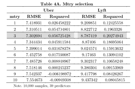
To select the appropriate number of predictors we run the ‘caret library’, this time, and unfortunately we have to reduce the sample for both firms to 10.000 since the computing cost with the sub-sample of 101,889 and 80,110 for Uber and Lyft respectively was not possible to run in the local computer. The computational time took approximately 25 min. We found in Table 4A, that the best ‘mtry’ selection is 3 for both samples.

library(caret)
set.seed(45)
trainub2 = sample_n(trainub, 10000, replace = F)
control <- trainControl(method='oob', search = 'grid')
tunegrid <- expand.grid(.mtry = (1:10)) 

# tunegrid for the whole sample
rf0 <- train(price ~., data = trainub2, method = 'rf',metric = 'RMSE', 
        tuneGrid = tunegrid, trControl = control)

Here’s the Table for the ‘mtry’ selection:

# Tunegrid only for most important 14 variables 
rf <- train(price ~ distance + source_Haymarket.Square+source_Beacon.Hill+
       source_Financial.District+ destination_Financial.District+
       destination_Beacon.Hill+ destination_Theatre.District+
       destination_Haymarket.Square+temperature+ windSpeed+
       destination_Back.Bay+visibility+ source_North.End+
       weekend, data = trainub2, method = 'rf',metric = 'RMSE', 
       tuneGrid = tunegrid, trControl = control)

# LYFT -----------------
trainly2 = sample_n(trainly, 10000, replace = F)
control <- trainControl(method='oob', search = 'grid')
tunegrid <- expand.grid(.mtry = (1:10)) 

# tunegrid for the whole sample
rfL0 <- train(price ~., data = trainly2, method = 'rf',metric = 'RMSE', 
     tuneGrid = tunegrid, trControl = control) 
# Tunegrid only for most important 14 variables 
rfL <- train(price ~ surge_multiplier+distance +temperature+visibility+temperature+
     source_Financial.District+ source_Haymarket.Square + 
     source_Beacon.Hill+destination_Back.Bay+
     destination_Beacon.Hill+ source_North.End+
     destination_South.Station+destination_Financial.District, 
    data = trainly2, method = 'rf',metric = 'RMSE', 
    tuneGrid = tunegrid, trControl = control)

par(mfrow=c(1,2))
plot(rf0)
plot(rfL)

As an example to compare different models, this time we only selected the most 14 important variables as predictors. For the tuning of mtry, we used two different set of variables, the first one includes all the variables -39 regressors-; while the second one, this includes only the most important 14 variables for both sub-samples. We found that the best mtry for this variable selection is equal to 2, we could expect this result, since this time the number of predictors have considerably decreased from 39 to 14. Results of the Second iteration are not shown.

Random Forest estimation: UBER

set.seed(45)
fit1 <- randomForest(price~., data=trainub, importance=TRUE, ntree=500, 
                maxnodes=25, mtry=3)
pred1 <- predict(fit1, testub)
test.err1=(mean(testub$price-pred1)^2)
set.seed(45)
fit11 <- randomForest(price~., data=trainub, importance=TRUE, ntree=700, 
              maxnodes=25, mtry=3)
pred2 <- predict(fit11, testub)
test.err2=(mean(testub$price-pred2)^2)
set.seed(45)
fit12 <- randomForest(price~., data=trainub, importance=TRUE, ntree=1000, 
                    maxnodes=25, mtry=3)
pred3 <- predict(fit12, testub)
test.err3=(mean(testub$price-pred3)^2)

oob = rbind(fit1$mse[500], fit11$mse[700], fit12$mse[1000])
err = rbind(test.err1, test.err2, test.err3)

matplot(c(500,700,1000), cbind(oob), pch=19 , col=c("red"),type="b",ylab="Mean Squared Error",xlab="Number of trees at each Split")
par(new=T)
matplot(1:3, cbind(err), pch=19 , col=c("blue"),type="b",xaxt = "n", yaxt = "n", xlab ='', ylab='')
legend("topright",legend=c("Out of Bag Error", 'Test error'),pch=19, col=c("red","blue"))
varImpPlot(fit11, pch=20, cex=.75, main='Best Random Forest')

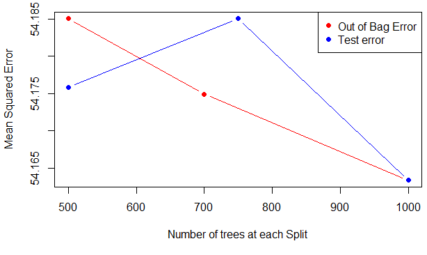
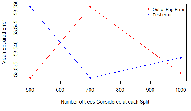
Here’s the plot the error test and MSE for Uber:

#----Random Forest Estimation: Lyft
set.seed(45)
fit1L <- randomForest(price~., data=trainly, importance=TRUE, ntree=500, 
        maxnodes=25, mtry=3)
pred1L <- predict(fit1L, testly)
test.err1L=(mean(testly$price-pred1L)^2)
set.seed(45)
fit2L <- randomForest(price~., data=trainly, importance=TRUE, ntree=700, 
                      maxnodes=25, mtry=3)
pred2L <- predict(fit2L, testly)
test.err2L=(mean(testly$price-pred2L)^2)
set.seed(45)
fit3L <- randomForest(price~., data=trainly, importance=TRUE, ntree=1000, 
                      maxnodes=25, mtry=3)
pred3L <- predict(fit3L, testly)
test.err3L=(mean(testly$price-pred3L)^2)

oobL = rbind(fit1L$mse[500], fit2L$mse[700], fit3L$mse[1000])
errL = rbind(test.err1L, test.err2L, test.err3L)

matplot(c(500,700,1000), cbind(oobL), pch=19, col=c("red"),type="b",ylab="Mean Squared Error",
        xlab="Number of trees considered at each Split")
par(new=T)
matplot(c(500,700,1000), cbind(errL), pch=19 , col=c("blue"),type="b",xaxt = "n", yaxt = "n", xlab ='', ylab='')
legend("topright",legend=c("Out of Bag Error", 'Test error'),pch=19, col=c("red","blue"))
varImpPlot(fit3L, pch=20, cex=.75, main='Best Random Forest')

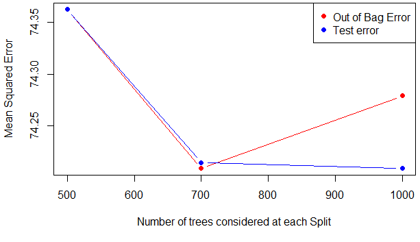
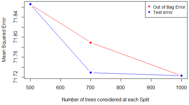
Here’s the plot the error test and MSE for Lyft:

Here’s the OOB error and Error test table:

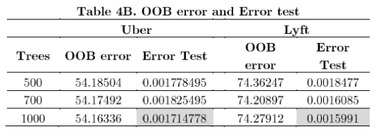
It is pretty clear that the smallest test errors are with 1,000 trees, although the smallest OOB error for Lyft is reached with 700 trees. For the next step of our analysis, we will use 1000 trees for Uber and only 700 for Lyft, the reason is that with 700 trees, both errors are small, if we consider 1000 trees, the OOB error increases. After the selection of trees we figures presenting the variables with more importance for each firm. Variables are ordered by %IncMSE, which shows an informative measure for the estimation of each variable.

library(ggplot2)

# VAR importance for Uber and Lyft

importance <- importance(fit12)
varImportance <- data.frame(Variables = row.names(importance), 
                            Importance = round(importance[,'%IncMSE'],2))
rankImportance <- varImportance %>% mutate(Rank = paste0('#',dense_rank(desc(Importance))))

ggplot(rankImportance, aes(x = reorder(Variables, Importance), 
                           y = Importance, fill = Importance)) + geom_bar(stat='identity') + 
    geom_text(aes(x = Variables, y = 0.5, label = Rank),
              hjust=0, vjust=0.55, size = 3, colour = 'white') +
    labs(x = 'Variables', size=5) +
    coord_flip() + ggtitle("Plot of variable importance for Uber")

# FOR LYFT -------------------------------------------------------

importance <- importance(fit2L)
varImportance <- data.frame(Variables = row.names(importance), 
                            Importance = round(importance[,'%IncMSE'],2))
rankImportance <- varImportance %>% mutate(Rank = paste0('#',dense_rank(desc(Importance))))

ggplot(rankImportance, aes(x = reorder(Variables, Importance), 
                           y = Importance, fill = Importance)) +
    geom_bar(stat='identity') + 
    geom_text(aes(x = Variables, y = 0.5, label = Rank),
              hjust=0, vjust=0.55, size = 3, colour = 'white') +
    labs(x = 'Variables') +
    coord_flip() + ggtitle("Plot of variable importance for Lyft")

par(mfrow=c(1,2))
plot(testub$price, pred3,
     xlab="observed",ylab="predicted", main='Initial prediction: Uber')
abline(a=1,b=1, col='red')
plot(testly$price, pred2L,
     xlab="observed",ylab="predicted", main='Initial prediction: Lyft')
abline(a=1,b=1, col='red')

Here’s the variable importance for Uber:

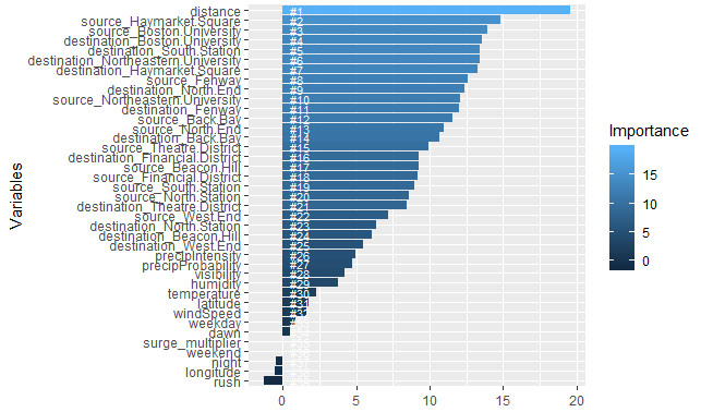
It is clear that the variables with more influence are: distance, Haymarket square, Boston University, South station, Northeastern University, North end and Back Bay. We can assume that Uber clients are young people or students, because Boston University & Northeastern University are among the places with more importance for pricing.

Here’s the variable importance for Lyft:

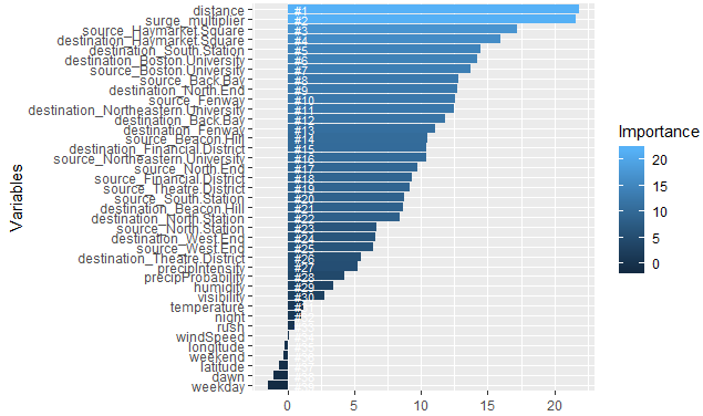
The variables with more influence are: distance, the surge multiplier, Haymarket square, Boston University, Back Bay and Fenway. Besides the places of destination and sources, we see that weather features don’t have any particular impact on pricing for the Random Forest technique.

R code for the Second iteration only with the best random forest

UBER

set.seed(45)
sec1=randomForest(price ~ distance + source_Haymarket.Square+source_Beacon.Hill+
    source_Financial.District+ destination_Financial.District+
    destination_Beacon.Hill+ destination_Theatre.District+
    destination_Haymarket.Square+temperature+ windSpeed+
   destination_Back.Bay+visibility+ source_North.End+
     weekend, data=trainub, mtry=2,ntree=500, importance=TRUE, maxnodes=25)
predsec1 <- predict(sec1, testub)
test.sec1=(mean(testub$price-predsec1)^2)
set.seed(45)
sec12=randomForest(price ~ distance + source_Haymarket.Square+source_Beacon.Hill+
         source_Financial.District+ destination_Financial.District+
        destination_Beacon.Hill+  destination_Theatre.District+
           destination_Haymarket.Square+temperature+ windSpeed+
        destination_Back.Bay+visibility+ source_North.End+
          weekend, data=trainub, mtry=2,ntree=700, importance=TRUE, maxnodes=25)
predsec2 <- predict(sec12, testub)
test.sec2=(mean(testub$price-predsec2)^2)
set.seed(45)
sec13=randomForest(price ~ distance + source_Haymarket.Square+source_Beacon.Hill+
      source_Financial.District+ destination_Financial.District+
    destination_Beacon.Hill+  destination_Theatre.District+
 destination_Haymarket.Square+temperature+ windSpeed+
    destination_Back.Bay+visibility+ source_North.End+
      weekend, data=trainub, mtry=2,ntree=1000, importance=TRUE, maxnodes=25)
predsec3 <- predict(sec13, testub)
test.sec3=(mean(testub$price-predsec3)^2)

oob1 = rbind(sec1$mse[500], sec12$mse[700],sec13$mse[1000])
err1 = rbind(test.sec3, test.sec1, test.sec2)

matplot(c(500,700,1000), cbind(oob1), pch=19 , col=c("red"),type="b",ylab="Mean Squared Error",xlab="Number of trees Considered at each Split")
par(new=T)
matplot(c(500,700,1000), cbind(err1), pch=19 , col=c("blue"),type="b",xaxt = "n", yaxt = "n", xlab ='', ylab='')
legend("topright",legend=c("Out of Bag Error", 'Test error'),pch=19, col=c("red","blue"),cex=0.9)

Here’s the plot the Error test and MSE for Uber - Second iteration:

LYFT

set.seed(45)
sec1L=randomForest(price ~ surge_multiplier+distance +temperature+visibility+temperature+
    source_Financial.District+ source_Haymarket.Square + source_Beacon.Hill+destination_Back.Bay+
     destination_Beacon.Hill+  source_North.End+destination_South.Station+destination_Financial.District,
     data=trainly, mtry=2,ntree=500, importance=T, maxnodes=25)
predsec1L <- predict(sec1L, testly)
test.sec1L=(mean(testly$price-predsec1L)^2)

set.seed(45)
sec2L=randomForest(price ~ surge_multiplier+distance +temperature+visibility+temperature+
     source_Financial.District+ source_Haymarket.Square + source_Beacon.Hill+destination_Back.Bay+
     destination_Beacon.Hill+  source_North.End+destination_South.Station+destination_Financial.District,
     data=trainly, mtry=2,ntree=700, importance=T, maxnodes=25)
predsec2L <- predict(sec2L, testly)
test.sec2L=(mean(testly$price-predsec2L)^2)

set.seed(45)
sec3L=randomForest(price ~ surge_multiplier+distance +temperature+visibility+temperature+
    source_Financial.District+ source_Haymarket.Square + source_Beacon.Hill+destination_Back.Bay+
    destination_Beacon.Hill+ source_North.End+destination_South.Station+destination_Financial.District,
    data=trainly, mtry=2,ntree=1000, importance=T, maxnodes=25)
predsec3L <- predict(sec3L, testly)
test.sec3L=(mean(testly$price-predsec3L)^2)

oob1L = rbind(sec1L$mse[500], sec2L$mse[700], sec3L$mse[1000])
err1L = rbind(test.sec1L, test.sec2L, test.sec3L)

matplot(c(500,700,1000), cbind(oob1L), pch=19 , col=c("red"),type="b",ylab="Mean Squared Error",xlab="Number of trees considered at each Split")
par(new=T)
matplot(c(500,700,1000), cbind(err1L), pch=19 , col=c("blue"),type="b",xaxt = "n", yaxt = "n", xlab ='', ylab='')
legend("topright",legend=c("Out of Bag Error", 'Test error'),pch=19, col=c("red","blue"), cex=0.9)

Here’s the plot the Error test and MSE for Lyft - Second iteration:

The OOB estimate of error rate is a useful measure to discriminate between different random forest classifiers. We could, for instance, vary the number of trees or the number of variables to be considered, and select the combination that produces the smallest value for this error rate. In that way, for the next step of our analysis, we will use again 1,000 trees for Uber and Lyft, the reason is that with 700 trees in Uber, the OOB error is the highest recorded and it could bias the output, and if we consider 1,000 trees, the error test increases a little, but not too much.

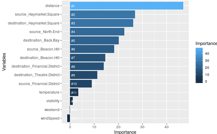
Variable importance with 1000 trees: UBER

importance <- importance(sec13)
varImportance <- data.frame(Variables = row.names(importance), 
                            Importance = round(importance[,'%IncMSE'],2))
rankImportance <- varImportance %>% mutate(Rank = paste0('#',dense_rank(desc(Importance))))

ggplot(rankImportance, aes(x = reorder(Variables, Importance), 
                           y = Importance, fill = Importance)) + geom_bar(stat='identity') + 
    geom_text(aes(x = Variables, y = 0.5, label = Rank),
              hjust=0, vjust=0.55, size = 3, colour = 'white') +
    labs(x = 'Variables', size=5) +
    coord_flip() + ggtitle("Variable importance: second iteration Uber")

par(mfrow=c(1,2))
plot(pred3,testub$price,
     xlab="predicted",ylab="actual", main='Initial prediction: Uber')
abline(a=8,b=1, col='red')
plot(predsec1,testub$price,
     xlab="predicted",ylab="actual", main='Second prediction: Uber')
abline(a=8,b=1, col='red')

Here’s the Variable importance for Uber - Second iteration:

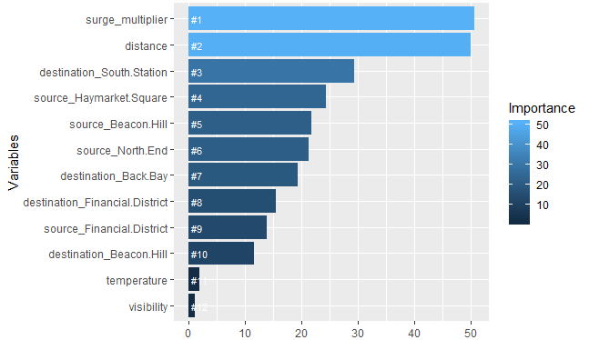
Variable importance with 1000 trees LYFT

importance <- importance(sec3L)
varImportance <- data.frame(Variables = row.names(importance), 
       Importance = round(importance[,'%IncMSE'],2))
rankImportance <- varImportance %>% mutate(Rank = paste0('#',dense_rank(desc(Importance))))

ggplot(rankImportance, aes(x = reorder(Variables, Importance), 
     y = Importance, fill = Importance)) + geom_bar(stat='identity') + 
    geom_text(aes(x = Variables, y = 0.5, label = Rank),
    hjust=0, vjust=0.55, size = 3, colour = 'white') +
    labs(x = 'Variables', size=5) +
    coord_flip() + ggtitle("Variable importance: second iteration Lyft")

Here’s the Variable importance for Lyft - Second iteration:

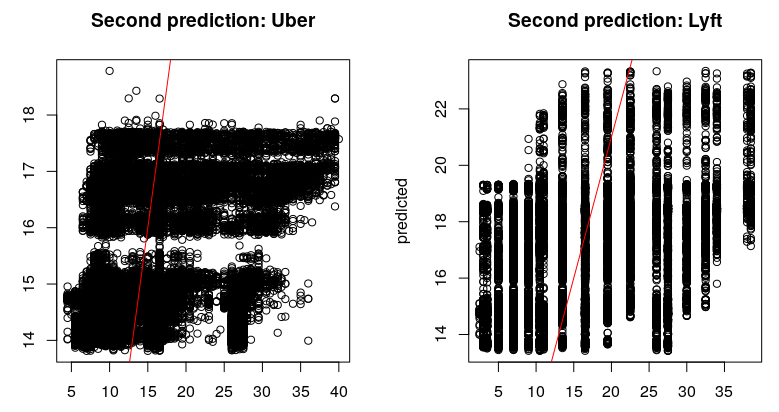
Second iteration prediction

par(mfrow=c(1,2))
plot(testub$price, predsec3,
     xlab="observed",ylab="predicted", main='Second prediction: Uber')
abline(a=1,b=1, col='red')
plot(testly$price,predsec3L,
     xlab="observed",ylab="predicted", main='Second prediction: Lyft')
abline(a=1,b=1, col='red')

dev.off()

Here’s the Prediction results for Uber and Lyft - Second iteration:

This is the end of part 4.