Trees

Tree classifiers in R

library(data.table)
library(tree)
library(readr)

NY <- read_delim("C:/Users/D/Desktop/NY.csv", ";", escape_double = FALSE, trim_ws = TRUE)
library(dplyr)
attach(NY)

NY$hp = as.factor(ifelse(NY$price <= 13.52, "Low", "High"))
NY$ub = as.factor(ifelse(NY$cab_type == 'Uber', "Uber", "Lyft"))

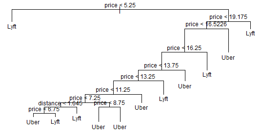
The first tree for the Uber and Lyft dataset

tree.di <- tree(ub ~ price+distance, data=NY)
summary(tree.di)
plot(tree.di)
text(tree.di, cex=.75)
title(main = "Unpruned Classification Tree")

Here’s the plot for our basic tree:

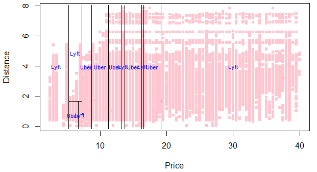
Plots partitions of tree

price.bi <- quantile(NY$price, 0:4/4)
cut.prices <- cut(NY$price, price.bi, include.lowest=TRUE)

plot(NY$price, NY$distance, col=hcl(10:2/11)[cut.prices], pch=15, 
     xlab="Price",ylab="Distance", main='Partition tree: Uber vs Lyft', cex=.75)
partition.tree(tree.di, ordvars=c("price","distance"), add=TRUE, col='blue', cex=.7)

plot(NY$price, NY$distance, col=hcl(10:2/11)[cut.prices], pch=15, 
     xlab="Price",ylab="Distance", main='Partition best tree', cex=.75)
partition.tree(tree.2, ordvars=c("price","distance"), add=TRUE, col='blue',cex=.7)

plot(NY$price, NY$distance, col=hcl(10:2/11)[cut.prices], pch=15, 
     xlab="Price",ylab="Distance", main='Partition pruneed tree', cex=.75)
partition.tree(pruned.tree, ordvars=c("price","distance"), add=TRUE, col='blue',cex=.7)

Here’s the partition plot for our basic tree:

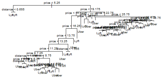
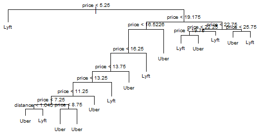
A more stylized tree mindev=0.001

tree.2 <- tree(ub ~ price+distance, data=NY, mindev=0.001)
summary(tree.2)
plot(tree.2)
text(tree.2, cex=.6)
title(main = "Unpruned Classification Tree")

Here’s the plot for our more stylized tree:

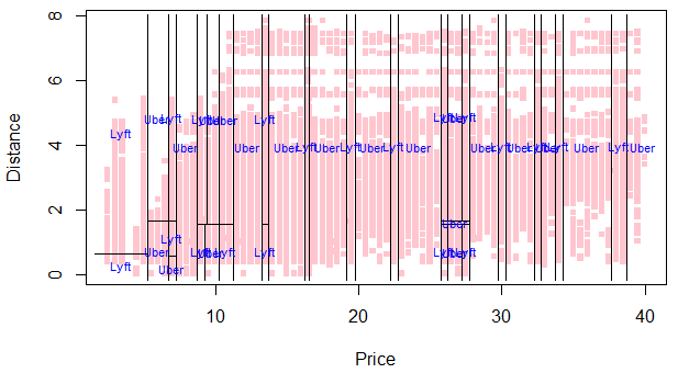
plot(NY$price, NY$distance, col=hcl(10:2/11)[cut.prices], pch=15, 
     xlab="Price",ylab="Distance", main='Pruned partition tree: Uber vs Lyft', 
     cex=.75)
partition.tree(pruned.tree, ordvars=c("price","distance"), add=TRUE)

Here’s the partition plot for our stylized tree:

Making the predictions

set.seed(45)
intrain  <- sample(1:nrow(NY), 0.7*nrow(NY))
trainny<- NY[intrain,]
testny  <- NY[-intrain,]

predt1 <- predict(tree.di, testny)
predt <- predict(tree.2, testny) # gives the probability for each class
head(predt)

Point prediction

Let’s translate the probability output to categorical output

maxidx <- function(arr) {
    return(which(arr == max(arr)))
}

idx <- apply(predt1, c(1), maxidx)
prediction <- c('Lyft', 'Uber')[idx]
table(prediction, testny$cab_type)

Another way to show the data: however it takes too much!!!

plot(NY$price, NY$distance, pch=19, col=as.numeric(NY$ub))
partition.tree(tree.di, label="cab_type", add=T)
legend("topleft",legend=unique(NY$cab_type), 
       col=unique(as.numeric(NY$cab_type)), pch=19) 

Prunned tree

pruned.tree <- prune.tree(tree.2, best=15)
plot(pruned.tree, )
text(pruned.tree, cex=.6)
title(main='Prunned best tree')
pruned.pre <- predict(pruned.tree, testny, type="class")
table(pruned.pre, testny$ub)

Here’s the plot for our prunned tree:

Here’s the partition plot for our prunned tree:

This package can also do K-fold cross-validation using cv.tree() to find the best tree: Here, let’s use all the variables and all the samples.

cv.model <- cv.tree(tree.2)
plot(cv.model)
title(main='CV best tree')

cv.model$dev
best.size <- cv.model$size[which(cv.model$dev==min(cv.model$dev))] 
best.size

cv.pruned <- prune.misclass(tree.2, best=35)
summary(cv.pruned)

predtcv <- predict(cv.pruned, testny)
head(predtcv)

idx <- apply(predtcv, c(1), maxidx)
prediction <- c('Lyft', 'Uber')[idx]
table(prediction, testny$cab_type)

Predictions and accuracy

trpred = predict(tree.2, trainny, type = "class")
tspred = predict(tree.2, testny, type = "class")

table(predicted = trpred, actual = trainny$ub)
table(predicted = tspred, actual = testny$ub)

accuracy = function(actual, predicted) {
    mean(actual == predicted)
}

Train accuracy

accuracy(predicted = trpred, actual = trainny$ub)

Test accuracy

accuracy(predicted = tspred, actual = testny$ub)

Accuracy results

	Train	Test
Stylized tree	0.7860975	0.7865336
Prunned tree	0.8778819	0.8764496

It is easy to see that the tree has been over-fit, and the test set performs slighlty better than the train set.

Cross Validation

We will now use cross-validation to find a tree by considering trees of different sizes which have been pruned from our original tree.

set.seed(45)
NYtree_cv = cv.tree(tree.2, FUN = prune.misclass)
plot(NYtree_cv)

Index of tree with minimum error

best.size2 <- NYtree_cv$size[which(NYtree_cv$dev==min(NYtree_cv$dev))] 
best.size2

Misclassification rate of each tree

NYtree_cv$dev/length(idx)
plot(NYtree_cv$size, NYtree_cv$dev/nrow(trainny), type = "b",
     xlab = "Tree Size", ylab = "CV Misclassification Rate")

Pruned tree

Train dataset

NYprune_trn = predict(pruned.tree, trainny, type = "class")
table(predicted = NYprune_trn, actual = trainny$ub)
accuracy(predicted = NYprune_trn, actual = trainny$ub)

Test dataset

NYprune_tst = predict(pruned.tree, testny, type = "class")
table(predicted = NYprune_tst, actual = testny$ub)
accuracy(predicted = NYprune_tst, actual = testny$ub)

The train set has performed almost as well as before, and there was a small improvement in the test set, but it is still obvious that we have over-fit.

Trees tend to do this. We will look at several ways to fix this, including: bagging, boosting and random forests, in the next posts.

This is the end of Part 3.