Xgb
XGboost
To conclude with the estimation part of the project we will use the Xgboost methodology to compare results with the previous estimations. Once again, due to time constraints and computing restrictions, we continue with the same size of the data sample from the two previous models only with the 14 variables with had more relative influence.
library(tidyverse)
library(xgboost)
library(caret)
library(dplyr)
trainub %>% select('price','distance', 'windSpeed','temperature','visibility','humidity',
'precipIntensity','destination_Back.Bay','source_Beacon.Hill','source_North.End',
'destination_Fenway', 'source_Back.Bay','source_Northeastern.University',
'destination_South.Station','source_Financial.District') -> trainub2
testub %>% select('price','distance', 'windSpeed','temperature','visibility','humidity',
    'precipIntensity','destination_Back.Bay','source_Beacon.Hill','source_North.End',
      'destination_Fenway', 'source_Back.Bay','source_Northeastern.University',
      'destination_South.Station','source_Financial.District') -> testub2

trainly %>% select('price','surge_multiplier','distance','windSpeed','visibility','temperature',
    'humidity','source_North.End','precipIntensity','destination_Back.Bay',
    'source_Boston.University','source_Beacon.Hill','source_North.Station',
    'source_Financial.District','source_Back.Bay') -> trainly2
testly %>% select('price','surge_multiplier','distance','windSpeed','visibility','temperature',
    'humidity','source_North.End','precipIntensity','destination_Back.Bay',
     'source_Boston.University','source_Beacon.Hill','source_North.Station',
     'source_Financial.District','source_Back.Bay') -> testly2
We use the xgboost & caret libraries, using xgbtree and gbm. As control parameters, we used CV only with 5 folds. But in the grid options we were more generous trying to tuning the best parameters for the booster parameters, with a maximum of 200 iterations, with a depth of the tree equal to (5, 10 and 15), with a learning rate (eta = 0.01), and with a length of 3 to the number of variables supplied to a tree.
1.) We estimate the model with XGBOOST with caret-XgbTree
Matrix sample for Uber
xub_train = xgb.DMatrix(as.matrix(trainub2 %>% select(-price)))
yub_train = trainub$price
xub_test = xgb.DMatrix(as.matrix(testub2 %>% select(-price)))
yub_test = testub$price
Matrix sample for Lyft
xly_train = xgb.DMatrix(as.matrix(trainly2 %>% select(-price)))
yly_train = trainly$price
xly_test = xgb.DMatrix(as.matrix(testly2 %>% select(-price)))
yly_test = testly$price
Control
xgb_trcontrol = trainControl( method = "cv",
    number = 5, allowParallel = T, verboseIter = F, returnData = F)
tune grid
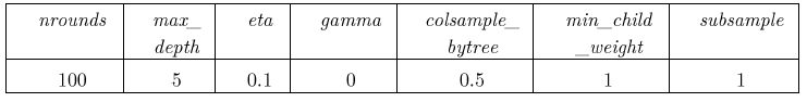
xgbGrid <- expand.grid(nrounds = c(100,200), max_depth = c(5,10,15),
     colsample_bytree = seq(0.5, 0.9, length.out = 3), eta = 0.1,
    gamma=0,  min_child_weight = 1, subsample = 1)
Here’s the Table for the Best tune - xgTree:
Running the model
set.seed(45)
xgbub_model = train(xub_train, yub_train,  trControl = xgb_trcontrol,
    tuneGrid = xgbGrid,  method = "xgbTree")

xgbly_model = train(xly_train, yly_train,  trControl = xgb_trcontrol,
    tuneGrid = xgbGrid, method = "xgbTree")

xgbub_model$bestTune
xgbly_model$bestTune
Evaluation
predi_ub = predict(xgbub_model, xub_test)
resid_ub = yub_test - predi_ub
RMSE = sqrt(mean(resid_ub^2))
cat('The root mean square error of the test data is ', round(RMSE,3),'\n')

predi_ly = predict(xgbly_model, xly_test)
resid_ly = yly_test - predi_ly
RMSE = sqrt(mean(resid_ly^2))
cat('The root mean square error of the test data is ', round(RMSE,3),'\n')
R2
yub_test_mean = mean(yub_test)
# Calculate total sum of squares
tss_ub =  sum((yub_test - yub_test_mean)^2 )
# Calculate residual sum of squares
rss_ub =  sum(resid_ub^2)
# Calculate R-squared
rsq_ub  =  1 - (rss_ub/tss_ub)
cat('The R-square of the test data is ', round(rsq_ub,3), '\n')

yly_test_mean = mean(yly_test)
# Calculate total sum of squares
tss_ly =  sum((yly_test - yly_test_mean)^2 )
# Calculate residual sum of squares
rss_ly =  sum(resid_ly^2)
# Calculate R-squared
rsq_ly  =  1 - (rss_ly/tss_ly)
cat('The R-square of the test data is ', round(rsq_ly,3), '\n')
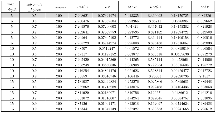
The best tune for both models (Uber and Lyft) is the same with 100 iterations, depth of tree equal to 5 and length of variables as 0.5. Below, Table 6B presents results on RMSE and R2, we found that the error is small for Uber as well as its R2, on the other hand, the model for Lyft shows a higher R2.
RMSE & R2
| Uber | Lyft | |
|---|---|---|
| RMSE | 7.396 | 8.55 |
| R2 | 0.042 | 0.093 |
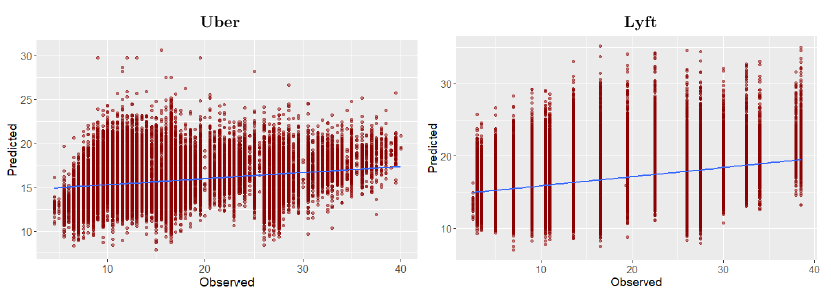
Finally, we present the prediction figures for Uber and Lyft.
Plot predictions vs test data : Uber
options(repr.plot.width=8, repr.plot.height=4)
ub_data = as.data.frame(cbind(predicted_ub = predi_ub,
                              observed_ub = yub_test))

ggplot(ub_data,aes(predicted_ub, observed_ub)) + geom_point(color = "darkred", alpha = 0.5) +
    geom_smooth(method=lm)+ ggtitle('Linear Regression ') + ggtitle("Extreme Gradient Boosting: Uber") +
    xlab("Predicted") + ylab("Observed") +
    theme(plot.title = element_text(color="darkgreen",size=16,hjust = 0.5),
          axis.text.y = element_text(size=12), axis.text.x = element_text(size=12,hjust=.5),
          axis.title.x = element_text(size=14), axis.title.y = element_text(size=14))
Plot predictions vs test data : Lyft
options(repr.plot.width=8, repr.plot.height=4)
ly_data = as.data.frame(cbind(predicted_ly = predi_ly,
                              observed_ly = yly_test))

ggplot(ly_data,aes(predicted_ly, observed_ly)) + geom_point(color = "darkred", alpha = 0.5) +
    geom_smooth(method=lm)+ ggtitle('Linear Regression ') + ggtitle("Extreme Gradient Boosting: Lyft") +
    xlab("Predicted") + ylab("Observed") +
    theme(plot.title = element_text(color="darkgreen",size=16,hjust = 0.5),
          axis.text.y = element_text(size=12), axis.text.x = element_text(size=12,hjust=.5),
          axis.title.x = element_text(size=14), axis.title.y = element_text(size=14))
Here’s the plots for Xgboost - model predictions:
Extra! GBM with caret
Concluding, although we already presented the gbm estimations in the above section, we found it interesting to reply to the exercise with another routine, at least to compare methodologies and of course, the most important results.
gbmGrid <-  expand.grid(interaction.depth = c(1,3,5,7,9),
   n.trees = c(50,100,150), shrinkage = 0.01, n.minobsinnode = 20)

gbm_ub <- caret::train(price ~ ., data = trainub2,
  method = "gbm", trControl = trainControl(method = "cv",
      number = 5,  verboseIter = FALSE), verbose = 0, tuneGrid = gbmGrid)

gbm_ly <- caret::train(price ~ ., data = trainly2,
     method = "gbm", trControl = trainControl(method = "cv",
      number = 5,  verboseIter = FALSE), verbose = 0, tuneGrid = gbmGrid)

gbm_ub$bestTune
gnm_ly$bestTune
Table fot the Best tune –caret::gbm-
| n.trees | interaction.depth | shrinkage | n.minobsinnode |
|---|---|---|---|
| 150 | 9 | 0.01 | 20 |
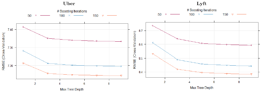
The best tune for both models (Uber and Lyft) is the same with 150 trees, interaction depth equal to 5 and ‘n.minobsinnode’ to 20. Regarding this last parameter, higher values mean smaller trees so make the algorithm run faster and use less memory, which may be a consideration. We believe results are not very sensitive to this parameter and given the stochastic nature of GBM performance it might actually be difficult to determine exactly what value is ‘the best’. We see that the small RMSE-CV is achieved with a 9 interaction depth and 150 iterations, Lyft’s results are similar to Uber.
Here’s the plots for Caret::gbm – best tune:
Evaluation for the model
predi_ub1 = predict(gbm_ub, testub2)
resid_ub1 = testub2$price - predi_ub1
RMSE = sqrt(mean(resid_ub1^2))
cat('The root mean square error of the test data is ', round(RMSE,3),'\n')

predi_ly1 = predict(gbm_ly, testly2)
resid_ly1 = testly2$price - predi_ly1
RMSE = sqrt(mean(resid_ly1^2))
cat('The root mean square error of the test data is ', round(RMSE,3),'\n')
Below, table presents results on RMSE and R2, we found that the gbm errors are s smaller than the xgbtree. So we could select this model prediction since it is the one that has the lower RMSE figures.
RMSE & R2
| Uber | Lyft | |
|---|---|---|
| RMSE | 7.292 | 8.391 |
| R2 | 0.069 | 0.126 |
trellis.par.set(caretTheme())
plot(gbm_ly)
plot(xgbub_model)

plot(gbm_ub, metric = "RMSE", plotType = "level", scales = list(x = list(rot = 90)))
plot(gbm_ly, metric = "RMSE", plotType = "level", scales = list(x = list(rot = 90)))
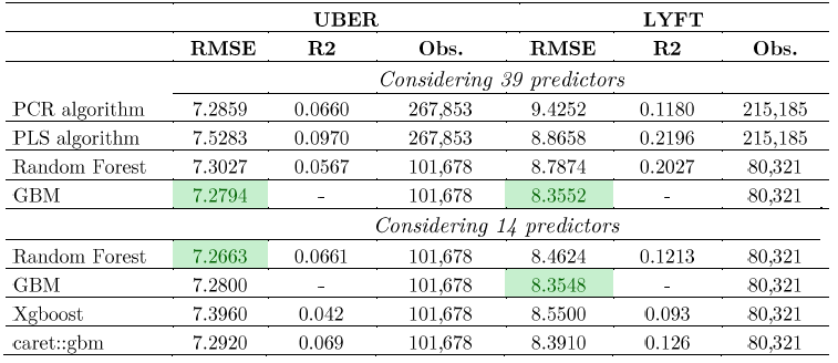
Finally, we gather all the metrics available during the exercise, which could help us to select the model with less error, of course, this will depend on the observation and the selected number of predictors. Results show that the model that has the smallest RMSE is GBM! The selection is consistent since it is chosen for almost all the exercises and for both firms. However, it appears that for Uber considering the subsample of 14 predictors, Random Forest is the best selection.
Selected metrics all models
This is the end pf part 6.