Ordinary Least Squares

5 minute read

Performing Linear Regression in Python

Importing the main libraries

import pandas as pd
import numpy as np
import matplotlib.pyplot as plt
from sklearn.model_selection import train_test_split
from sklearn.linear_model import LinearRegression

"""
Dataframe needs to be a pd.DataFrame
"""

def clean_dataset(df):
    assert isinstance(df, pd.DataFrame), 
    df.dropna(inplace=True)
    indices_to_keep = ~df.isin([np.nan, np.inf, -np.inf]).any(1)
    return df[indices_to_keep]

After defining our function to clean NAs and Inf observations and take a subsample considering only of the numerical variables.

df = pd.read_csv("rus2.csv", sep=",")

dt = df.select_dtypes(include=np.number)
clean_dataset(dt)
dt.head(6)

y = dt["price_usd"].values
x = dt.drop(["price_usd"], axis=1)

After that we define the xand y variables, where y is the car service price is $US.

Following, we will use the Statsmodels package to estimate the linear model, in that way we estimate three set of regressions, the first considers all the variables, the second takes: ‘total_time’,’wait_time’,’surge_multiplier’,’driver_gender’,’distance_kms’, and the third considers only: ‘wait_time’,’surge_multiplier’,’driver_gender’,’distance_kms’.

import statsmodels.api as sm

reg1 = sm.OLS(endog = y, exog = x).fit()
reg1.summary()

x2 = ['total_time','surge_multiplier','driver_gender','distance_kms' ]
x = sm.add_constant(x)
reg2 = sm.OLS(endog = y, exog = x[x2]).fit()
reg2.summary()

x3 = ['wait_time','surge_multiplier','driver_gender','distance_kms' ]
# x = sm.add_constant(x)
reg3 = sm.OLS(endog = y, exog = x[x3]).fit()
reg3.summary()

Below we define a nice function to gather all the results in one table.

from statsmodels.iolib.summary2 import summary_col
dict={'No. observations' : lambda x: f"{int(x.nobs):d}"}

results_table = summary_col(results=[reg1,reg2,reg3], float_format='%0.3f',
                            stars = True, model_names=['Model 1',
                                         'Model 2',
                                         'Model 3'],
                            info_dict=dict, regressor_order= ['surge_multiplier','driver_gender','distance_kms','total_time',
                            'wait_time', 'humidity', 'temperature_value','wind_speed'])

results_table.add_title('Table 1 - OLS Regressions')
print(results_table)

But, there are simple ways to do it better and simple.

from stargazer.stargazer import Stargazer
from IPython.core.display import HTML

ht = Stargazer([reg1, reg2, reg3])
HTML(ht.render_html())

From the results of Table 1, we can see that considering all the variables, the temperature and wind speed are not statistically significant, but appears that higher humidity have a negative effect on price; on the other hand, considering the models 2 and 3, in they we omit the environmental variables, in model 2 we consider only Total time of the trip, and in Model 3 we use the Wait time of the passenger.

From columns of 2 and 3, we see that only the Total time still has a positive impact on price, however when we use Wait time we see that the variable is not significant anymore.

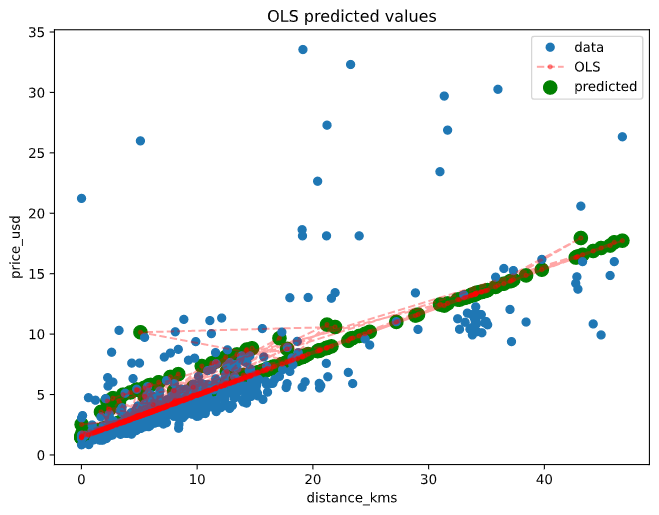
Finally, we define a plot where we can see the OLS estimations and all the predicted points by the selected regression model, in this case the prediction use the the third model.

           Table 1 - OLS Regressions
===============================================
                   Model 1   Model 2   Model 3 
-----------------------------------------------
surge_multiplier  4.640***  3.173***  3.640*** 
                  (0.739)   (0.583)   (0.578)  
driver_gender     -1.871*** -2.283*** -2.232***
                  (0.585)   (0.580)   (0.586)  
distance_kms      0.288***  0.315***  0.349*** 
                  (0.018)   (0.015)   (0.013)  
total_time        0.059***  0.031***           
                  (0.012)   (0.008)            
wait_time         -0.054***           0.009    
                  (0.019)             (0.013)   
humidity          -2.398***                    
                  (0.683)                      
temperature_value -0.012                       
                  (0.012)                      
wind_speed        -0.026                       
                  (0.061)                      
No. observations  643       643       643
R-squared         0.826     0.821     0.817    
                  0.828     0.822     0.818 
===============================================
Standard errors in parentheses.
* p<.1, ** p<.05, ***p<.01

Finally we define a simpler plot when we can see the OLS estimations and all the predicted points by the selected regression model.

## PLOT

from statsmodels.sandbox.regression.predstd import wls_prediction_std
prstd, iv_u, il_v = wls_prediction_std(reg2)

fig, ax = plt.subplots(figsize=(8,6))

ax.plot(x.distance_kms, y, 'o', label="data")

ax.scatter(dt['distance_kms'], reg3.predict(), label='predicted', color='green',  s=100)
ax.plot(x.distance_kms, reg3.fittedvalues, 'r--.', label="OLS", alpha=0.35)

ax.legend(loc='best')
ax.set_title('OLS predicted values')
ax.set_xlabel('distance_kms')
ax.set_ylabel('price_usd')
plt.show()

Here’s the plot for the OLS model with predicted values : alt

Twitter Facebook LinkedIn